Today I want to test some ways to deal with implicit missing values: namely, creating grids with several commands and performing full joins on our data. Let’s use again COVID-19 vaccinations data in Italy, available from the official repo.
Load Data
url_vaccinations <-
  'https://raw.githubusercontent.com/italia/covid19-opendata-vaccini/master/dati/somministrazioni-vaccini-latest.csv'

read_csv(url_vaccinations,
         col_types = cols(
           # parse as dates
           data_somministrazione = "D",
           # parse as factors
           fornitore = "f",
           area = "f",
           fascia_anagrafica = "f"
           # the rest, let it be guessed
         )) %>%
  # remove 'categoria' from several column names
  rename_with( ~ stringr::str_remove(.x, 'categoria_')) %>%
  # shorten some other variable names
  rename(
    operatori_sanitari = operatori_sanitari_sociosanitari,
    data = data_somministrazione
  ) %>%
  # create a new column with total vaccinations
  mutate(nuovi_vaccinati = sesso_maschile + sesso_femminile) %>%
  # reorder columns
  relocate(nuovi_vaccinati, .after = 'fascia_anagrafica') ->
  vaccinations

vaccinations %>% head(9)
## # A tibble: 9 x 17
## data fornitore area fascia_anagrafi… nuovi_vaccinati sesso_maschile
## <date> <fct> <fct> <fct> <dbl> <dbl>
## 1 2020-12-27 Pfizer/B… ABR 20-29 1 1
## 2 2020-12-27 Pfizer/B… ABR 30-39 4 1
## 3 2020-12-27 Pfizer/B… ABR 40-49 7 1
## 4 2020-12-27 Pfizer/B… ABR 50-59 9 4
## 5 2020-12-27 Pfizer/B… ABR 60-69 14 10
## 6 2020-12-27 Pfizer/B… ABR 70-79 1 1
## 7 2020-12-27 Pfizer/B… ABR 80-89 1 1
## 8 2020-12-27 Pfizer/B… BAS 20-29 9 4
## 9 2020-12-27 Pfizer/B… BAS 30-39 28 10
## # … with 11 more variables: sesso_femminile <dbl>, operatori_sanitari <dbl>,
## # personale_non_sanitario <dbl>, ospiti_rsa <dbl>, over80 <dbl>,
## # prima_dose <dbl>, seconda_dose <dbl>, codice_NUTS1 <chr>,
## # codice_NUTS2 <chr>, codice_regione_ISTAT <dbl>, nome_area <chr>Create Grids
To fill implicit missing values, we need to check against every possible combinations of factors and dates in our data. This means creating a grid and then performing a full join.
expand_grid(
    data = seq.Date(from = min(vaccinations$data),
                    to = max(vaccinations$data),
                    by = 'day'),
    area = forcats::fct_unique(vaccinations$area),
    fornitore = forcats::fct_unique(vaccinations$fornitore),
    fascia_anagrafica = forcats::fct_unique(vaccinations$fascia_anagrafica),
  ) %>% head()
## # A tibble: 6 x 4
## data area fornitore fascia_anagrafica
## <date> <fct> <fct> <fct>
## 1 2020-12-27 ABR Pfizer/BioNTech 20-29
## 2 2020-12-27 ABR Pfizer/BioNTech 30-39
## 3 2020-12-27 ABR Pfizer/BioNTech 40-49
## 4 2020-12-27 ABR Pfizer/BioNTech 50-59
## 5 2020-12-27 ABR Pfizer/BioNTech 60-69
## 6 2020-12-27 ABR Pfizer/BioNTech 70-79The same can be achieved in this way:
vaccinations %>%
  expand(
    # create a full sequence between the first and last date
    full_seq(data, 1),
    area, fornitore, fascia_anagrafica)
## # A tibble: 13,608 x 4
## `full_seq(data, 1)` area fornitore fascia_anagrafica
## <date> <fct> <fct> <fct>
## 1 2020-12-27 ABR Pfizer/BioNTech 20-29
## 2 2020-12-27 ABR Pfizer/BioNTech 30-39
## 3 2020-12-27 ABR Pfizer/BioNTech 40-49
## 4 2020-12-27 ABR Pfizer/BioNTech 50-59
## 5 2020-12-27 ABR Pfizer/BioNTech 60-69
## 6 2020-12-27 ABR Pfizer/BioNTech 70-79
## 7 2020-12-27 ABR Pfizer/BioNTech 80-89
## 8 2020-12-27 ABR Pfizer/BioNTech 90+
## 9 2020-12-27 ABR Pfizer/BioNTech 16-19
## 10 2020-12-27 ABR Moderna 20-29
## # … with 13,598 more rowsMuch neater, uh? Still, there are very many values and once the data gets larger it will take some more time.
vaccinations %>%
  full_join(vaccinations %>% expand(data, area, fornitore, fascia_anagrafica),
            by = c('data', 'area', 'fornitore', 'fascia_anagrafica')) %>%
  # sort data
  arrange(area, data) %>%
  # replace NAs that popped up
  mutate(across(where(is.numeric), ~ replace_na(.x, 0))) %>%
  # don't know why it does not work
  mutate(fascia_anagrafica = fct_inorder(fascia_anagrafica)) -> vaccinations_ita

vaccinations_ita %>% head(10)
## # A tibble: 10 x 17
## data fornitore area fascia_anagrafi… nuovi_vaccinati sesso_maschile
## <date> <fct> <fct> <fct> <dbl> <dbl>
## 1 2020-12-27 Pfizer/B… ABR 20-29 1 1
## 2 2020-12-27 Pfizer/B… ABR 30-39 4 1
## 3 2020-12-27 Pfizer/B… ABR 40-49 7 1
## 4 2020-12-27 Pfizer/B… ABR 50-59 9 4
## 5 2020-12-27 Pfizer/B… ABR 60-69 14 10
## 6 2020-12-27 Pfizer/B… ABR 70-79 1 1
## 7 2020-12-27 Pfizer/B… ABR 80-89 1 1
## 8 2020-12-27 Pfizer/B… ABR 90+ 0 0
## 9 2020-12-27 Pfizer/B… ABR 16-19 0 0
## 10 2020-12-27 Moderna ABR 20-29 0 0
## # … with 11 more variables: sesso_femminile <dbl>, operatori_sanitari <dbl>,
## # personale_non_sanitario <dbl>, ospiti_rsa <dbl>, over80 <dbl>,
## # prima_dose <dbl>, seconda_dose <dbl>, codice_NUTS1 <chr>,
## # codice_NUTS2 <chr>, codice_regione_ISTAT <dbl>, nome_area <chr>This is a very great deal of observations, and as of this day there are more missing values than complete ones. This is because Moderna started deliveries more than two weeks later than Pfizer/BioNTech (as the European Center for Disease Prevention and Control approved the vaccine later) and there were also some days between the start of the campaign and approximately January 10th where no vaccines administered.
Now we want to create some smaller datasets to be able to streamline visualisations later.
Group Data by Age Range
Let’s group the data by data, fornitore and fascia_anagrafica to see how vaccinations proceed within the same population range. Furthermore, compute the cumulative totals for each numeric variable.
vaccinations_ita %>%
  group_by(data, fascia_anagrafica, fornitore) %>%
  summarise(across(where(is.numeric), sum)) %>%
  mutate(across(where(is.numeric), list(totale = ~ cumsum(.x)))) %>%
  arrange(data, fornitore) %>%
  rename(vaccinati_totale = nuovi_vaccinati_totale) -> vaccinations_by_age_ita

vaccinations_by_age_ita %>% head()
## # A tibble: 6 x 23
## # Groups: data, fascia_anagrafica [6]
## data fascia_anagrafi… fornitore nuovi_vaccinati sesso_maschile
## <date> <fct> <fct> <dbl> <dbl>
## 1 2020-12-27 20-29 Pfizer/B… 640 236
## 2 2020-12-27 30-39 Pfizer/B… 1023 458
## 3 2020-12-27 40-49 Pfizer/B… 1428 537
## 4 2020-12-27 50-59 Pfizer/B… 2112 893
## 5 2020-12-27 60-69 Pfizer/B… 1429 1036
## 6 2020-12-27 70-79 Pfizer/B… 129 87
## # … with 18 more variables: sesso_femminile <dbl>, operatori_sanitari <dbl>,
## # personale_non_sanitario <dbl>, ospiti_rsa <dbl>, over80 <dbl>,
## # prima_dose <dbl>, seconda_dose <dbl>, codice_regione_ISTAT <dbl>,
## # vaccinati_totale <dbl>, sesso_maschile_totale <dbl>,
## # sesso_femminile_totale <dbl>, operatori_sanitari_totale <dbl>,
## # personale_non_sanitario_totale <dbl>, ospiti_rsa_totale <dbl>,
## # over80_totale <dbl>, prima_dose_totale <dbl>, seconda_dose_totale <dbl>,
## # codice_regione_ISTAT_totale <dbl>What to do with this?
Before moving on to grouping the data, let’s see how many people by age range received a shot (and from which supplier) by age range over time.
vaccinations_by_age_ita %>%
  ggplot(aes(data, nuovi_vaccinati, fill = fornitore)) +
  geom_col() +
  facet_wrap(~ fascia_anagrafica) +
  scale_fill_viridis_d(begin = 0.75, end = 0.25) +
  theme_minimal()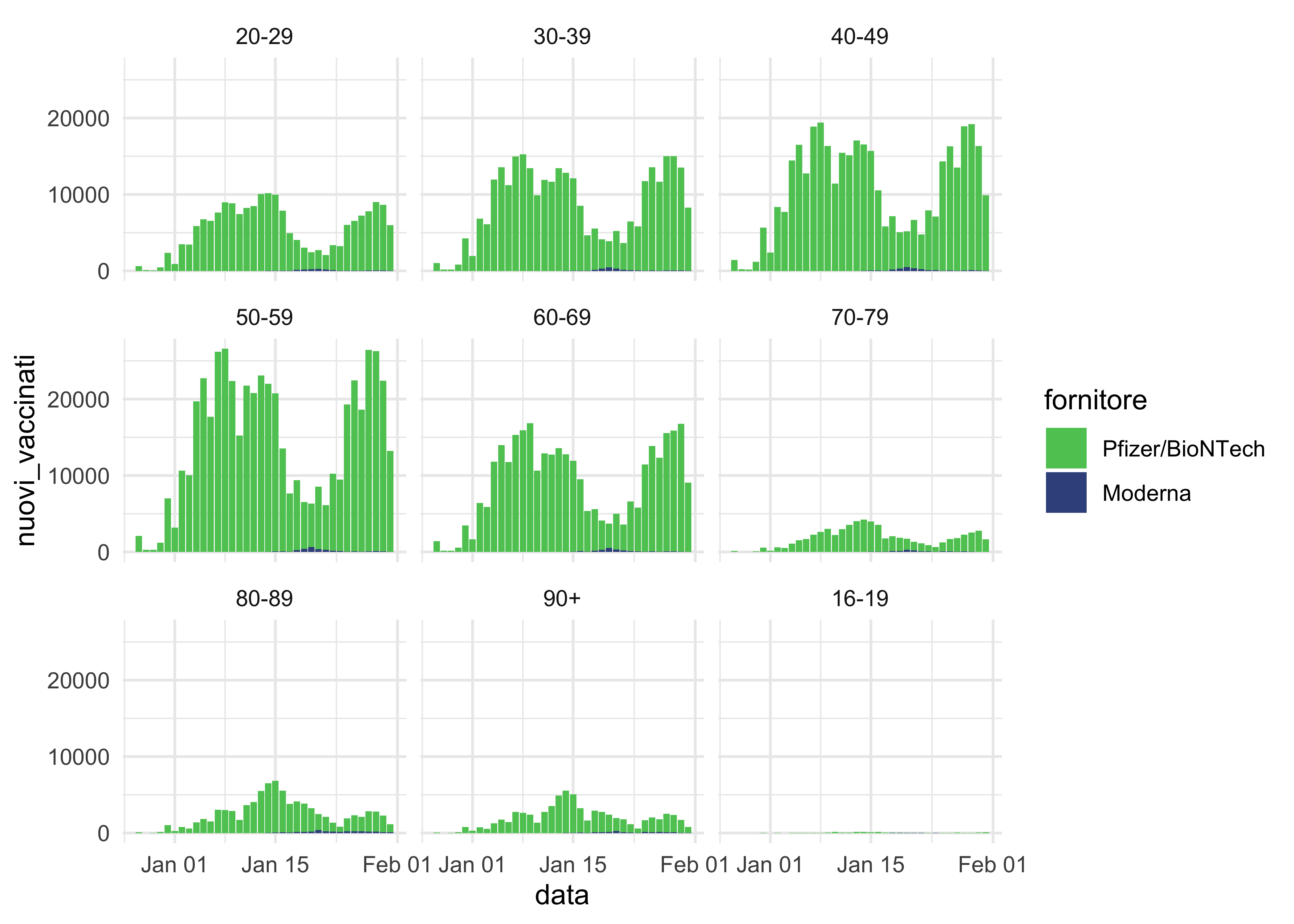
We can also obtain the totals by age range:
vaccinations_by_age_ita %>%
  # remove cumulative sums, as they will be obtained via `summarise`:
  select(1:12) %>%
  group_by(fascia_anagrafica, fornitore) %>%
  summarise(across(where(is.numeric), sum)) %>%
  rename(vaccinati_totale = nuovi_vaccinati) -> totals_by_age_ita

totals_by_age_ita %>% head()
## # A tibble: 6 x 11
## # Groups: fascia_anagrafica [3]
## fascia_anagrafi… fornitore vaccinati_totale sesso_maschile sesso_femminile
## <fct> <fct> <dbl> <dbl> <dbl>
## 1 20-29 Pfizer/B… 193924 65151 128773
## 2 20-29 Moderna 1427 578 849
## 3 30-39 Pfizer/B… 308332 121179 187153
## 4 30-39 Moderna 1897 807 1090
## 5 40-49 Pfizer/B… 383252 125121 258131
## 6 40-49 Moderna 2332 1025 1307
## # … with 6 more variables: operatori_sanitari <dbl>,
## # personale_non_sanitario <dbl>, ospiti_rsa <dbl>, over80 <dbl>,
## # prima_dose <dbl>, seconda_dose <dbl>See how first and second shots are distributed by age range and supplier. Arguably, this is not very informative. But let’s wait a couple of months: I bet it will prove useful!
totals_by_age_ita %>%
  # we don't need all of these columns
  select(fascia_anagrafica, fornitore, prima_dose, seconda_dose) %>%
  # shift to long format and exclude cols that can't be pivoted
  pivot_longer(!c(fascia_anagrafica, fornitore),
               # give names to the new cols
               names_to = 'values',
               values_to = 'counts') %>%
  ggplot(aes(fornitore, counts, fill = values)) +
  geom_col() +
  facet_wrap(~ fascia_anagrafica) +
  scale_fill_viridis_d(begin = 0.55, end = 0.95) +
  theme_minimal() +
  labs(
    title = 'Number of shots by supplier, per age range',
    x = 'date',
    y = NULL,
    fill = NULL
  ) +
  theme(legend.position = 'bottom')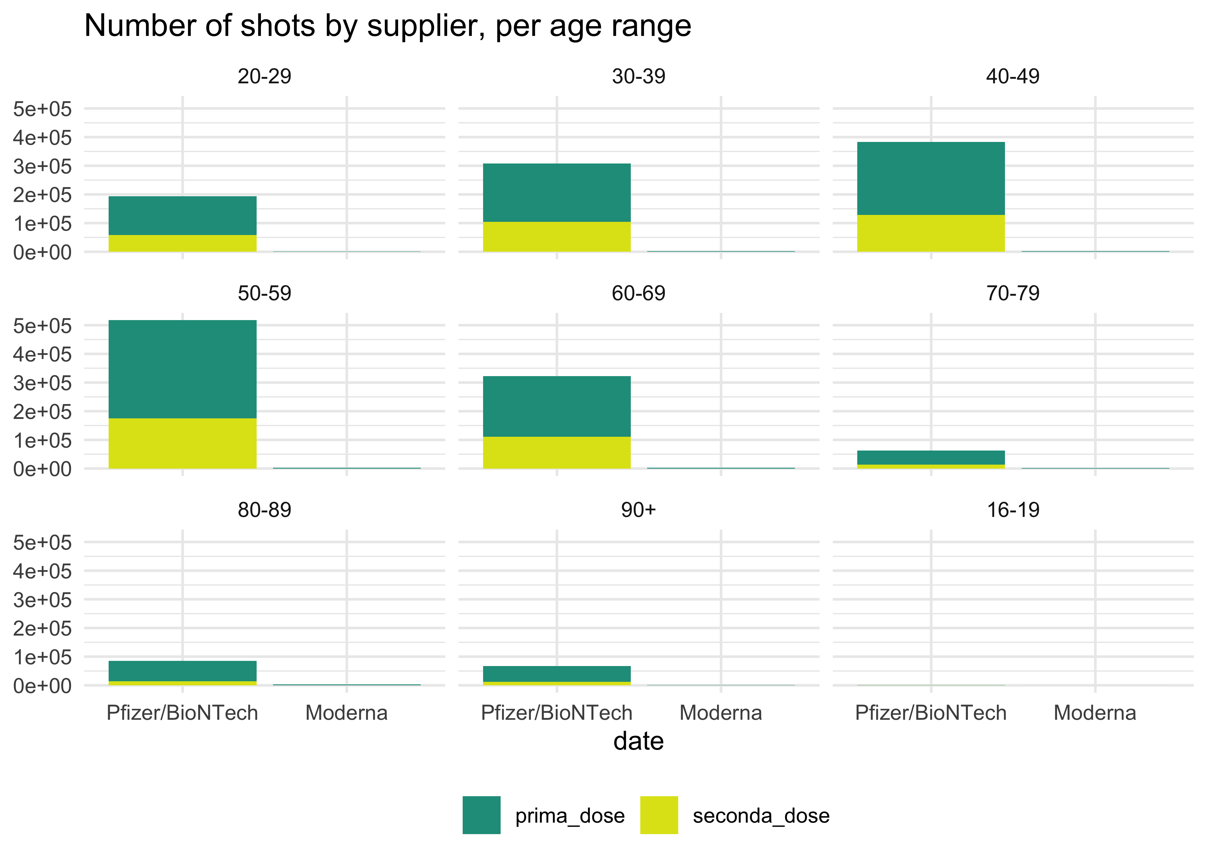
We can also picture the data as percentages:
totals_by_age_ita %>%
  # we don't need all of these columns
  mutate(across(
    # across these two cols
    c(prima_dose, seconda_dose),
    # the new cols will be called {colname}.pct
    list(pct = ~ .x / (prima_dose + seconda_dose))
  )) %>%
  select(fascia_anagrafica, fornitore, prima_dose_pct, seconda_dose_pct) %>%
  # shift to long format and exclude cols that can't be pivoted
  pivot_longer(!c(fascia_anagrafica, fornitore),
               # give names to the new cols
               names_to = 'values',
               values_to = 'counts') %>%
  ggplot(aes(fornitore, counts, fill = values)) +
  geom_col() +
  facet_wrap(~ fascia_anagrafica) +
  scale_fill_viridis_d(begin = 0.55, end = 0.95) +
  scale_y_continuous(labels = scales::percent) +
  theme_minimal() +
  labs(
    title = '% of shots by supplier, per age range',
    x = 'date',
    y = NULL,
    fill = NULL
  ) +
  theme(legend.position = 'bottom')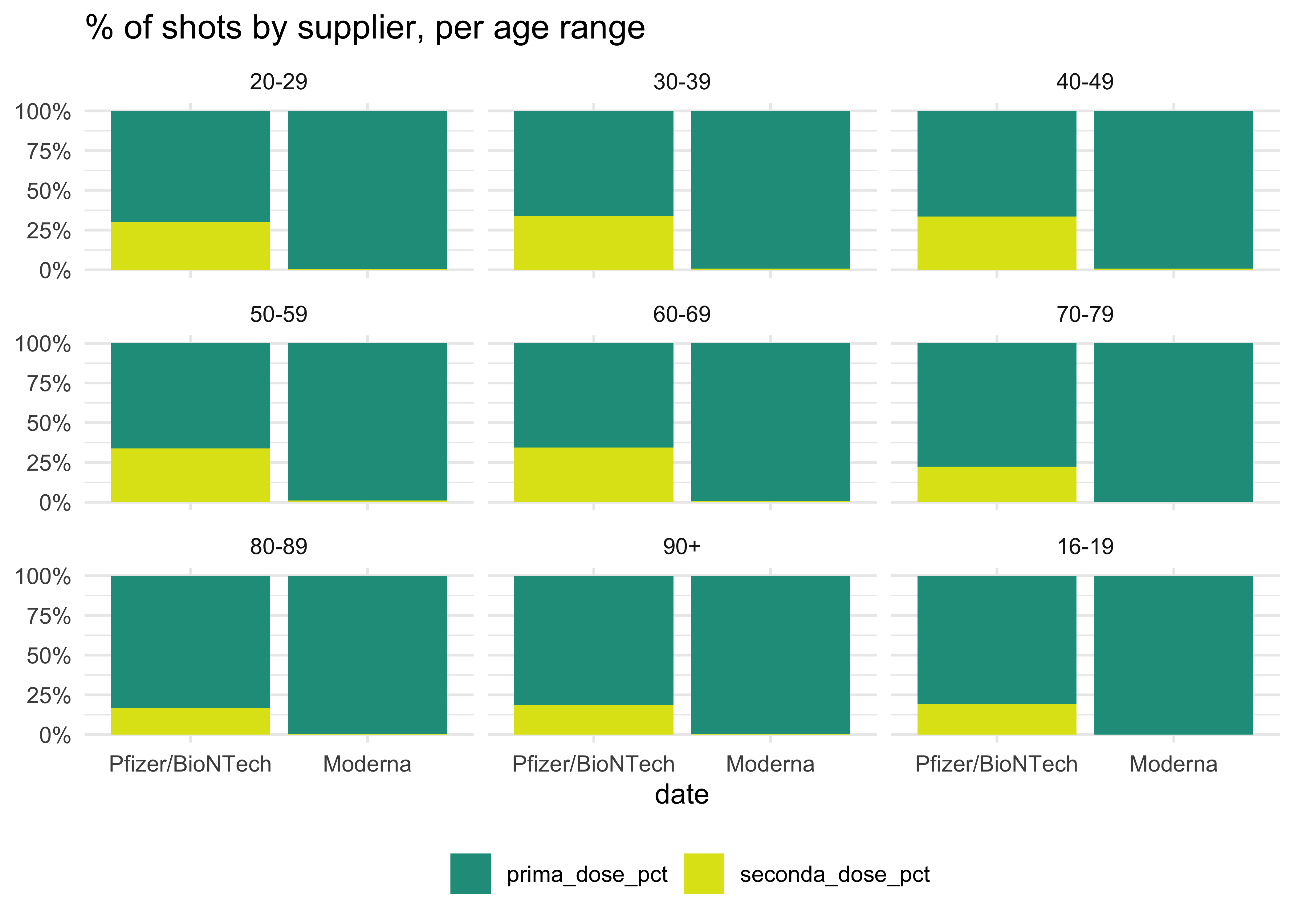
Does it really tell something? Well, it might not. But these posts are meant to document the process to find the better one and, of course, practice! We can do better using the time series data:
vaccinations_by_age_ita %>%
  select(data, fascia_anagrafica, fornitore, prima_dose, seconda_dose) %>%
  pivot_longer(
    !c(data,fascia_anagrafica, fornitore),
    names_to = 'values',
    values_to = 'counts'
  ) %>%
  ggplot(aes(data, counts, fill = values)) +
  geom_col() +
  facet_wrap(~ fascia_anagrafica) +
  scale_fill_viridis_d(begin = 0.55, end = 0.95) +
  theme_minimal() +
  labs(
    title = 'Vaccine Shots by Age Range',
    x = 'date',
    y = NULL,
    fill = NULL
  ) +
  theme(legend.position = 'bottom')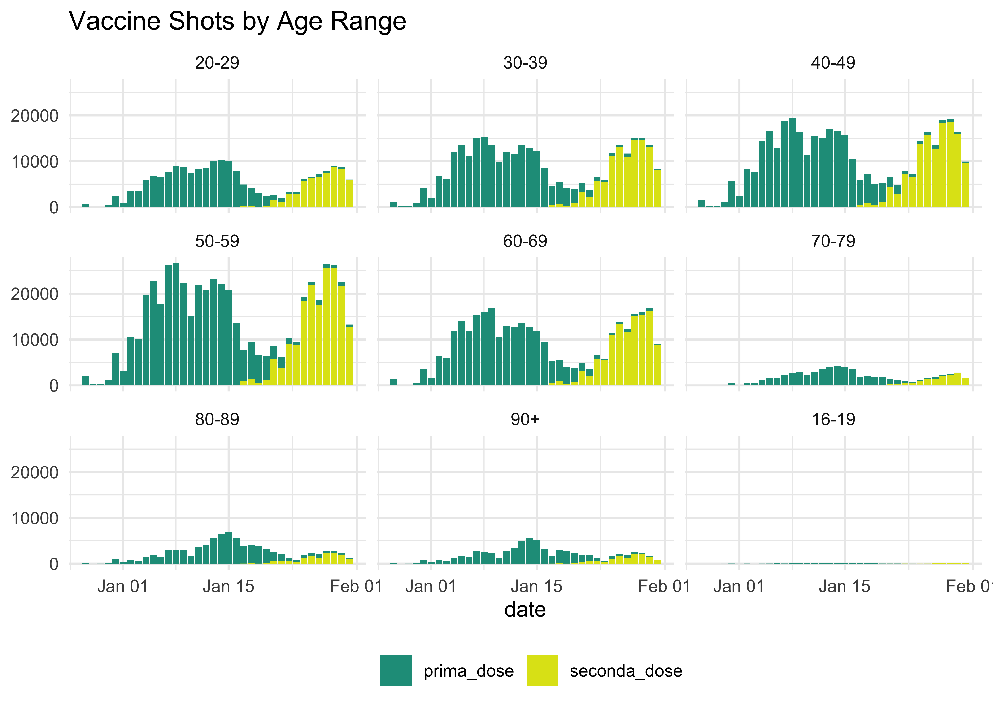
This does not tell much either: the additional dimension of the doses is not enriched by these additional dimensions (but it’s pretty good looking, is it not?).
Group Data By Area
Let’s wrap up by grouping the data by area.
vaccinations_ita %>%
  group_by(data, area, fornitore) %>%
  # create new columns with the sum of the grouped rows
  summarise(across(where(is.numeric), sum)) %>%
  # reorder
  relocate(nuovi_vaccinati, .after = area) %>%
  # create new rows with cumulative sums
  mutate(across(where(is.numeric), list(totale = ~ cumsum(.x)))) %>%
  rename(vaccinati_totale = nuovi_vaccinati_totale) %>%
  arrange(area) -> vaccinations_by_area_ita
Before grouping again to get the totals, we want to enrich this data with the population and deliveries data. This script is a bit more elaborate:
read_csv(
  'https://raw.githubusercontent.com/orizzontipolitici/covid19-vaccine-data/main/data_ita/doses_by_area_ita.csv'
) -> doses_by_area

vaccinations_by_area_ita %>%
  # `doses_by_area` is wide in format: we don't need `fornitore`
  select(1:12, -fornitore) %>%
  group_by(area) %>%
  summarise(across(where(is.numeric), sum)) %>%
  rename(vaccinati_totale = nuovi_vaccinati) %>%
  # also, it has the column for Italy, so we have to add one new line
  add_row(area = 'ITA',
          # the `.` indicates the object itself!
          vaccinati_totale = sum(.$vaccinati_totale),
          sesso_maschile = sum(.$sesso_maschile),
          sesso_femminile = sum(.$sesso_femminile),
          operatori_sanitari = sum(.$operatori_sanitari),
          personale_non_sanitario = sum(.$personale_non_sanitario),
          ospiti_rsa = sum(.$ospiti_rsa),
          over80 = sum(.$over80),
          prima_dose = sum(.$prima_dose),
          seconda_dose = sum(.$seconda_dose),
  ) %>%
  # perform inner join by area!
  inner_join(doses_by_area, by = 'area') %>%
  relocate(
    nome, NUTS2, area, popolazione_2020
  ) %>%
  # create new columns:
  mutate(
    # vaccinated each 1000 people
    vaccinati_ogni_mille = round(vaccinati_totale / popolazione_2020 * 1000, digits = 2),
    # share of vaccines used out of all received
    percent_vaccini_usati = round(vaccinati_totale / totale_dosi * 100, digits = 2)
  ) -> totals_by_area_ita

totals_by_area_ita
## # A tibble: 22 x 19
## nome NUTS2 area popolazione_2020 vaccinati_totale sesso_maschile
## <chr> <chr> <chr> <dbl> <dbl> <dbl>
## 1 Abru… ITF1 ABR 1293941 29268 10722
## 2 Basi… ITF5 BAS 553254 16609 6735
## 3 Cala… ITF6 CAL 1894110 42925 20822
## 4 Camp… ITF3 CAM 5712143 175906 85039
## 5 Emil… ITH5 EMR 4464119 195438 65908
## 6 Friu… ITH4 FVG 1206216 49170 16461
## 7 Lazio ITI4 LAZ 5755700 186682 72315
## 8 Ligu… ITC3 LIG 1524826 52122 18426
## 9 Lomb… ITC4 LOM 10027602 299631 98518
## 10 Marc… ITI3 MAR 1512672 42841 15369
## # … with 12 more rows, and 13 more variables: sesso_femminile <dbl>,
## # operatori_sanitari <dbl>, personale_non_sanitario <dbl>, ospiti_rsa <dbl>,
## # over80 <dbl>, prima_dose <dbl>, seconda_dose <dbl>, totale_pfizer <dbl>,
## # totale_moderna <dbl>, totale_dosi <dbl>, dosi_ogni_mille <dbl>,
## # vaccinati_ogni_mille <dbl>, percent_vaccini_usati <dbl>